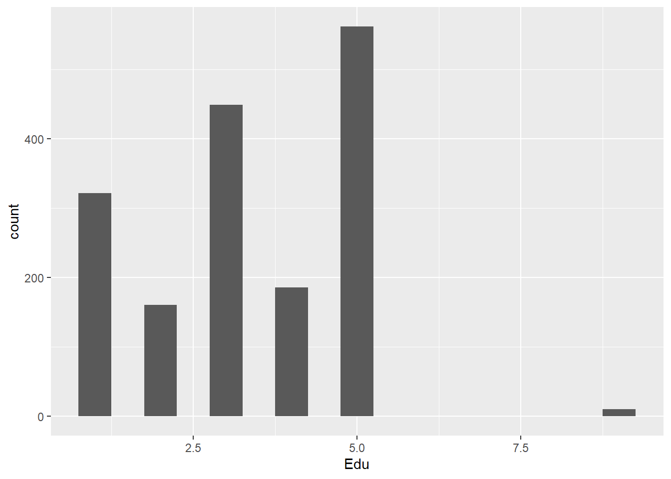
9 = ?????? Assume that is a numerical error, 9 does not seem to be defined in the dataset
The values seem to most often congregate around senior high education and 5, which an educated assumption could be made that it is Masters/Graduate Education.
Problems Encountered
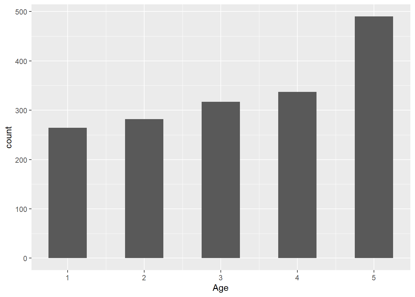
A significant problem with the data set is the lack of definitions for certain values. For example, in the age range response values 1-4 are defined, but 5 is not. For the education response range, 1-4 are again defined, but 5/6 are not defined (and for some reason a 9 exists).
As a result of this, it is much more difficult to properly interpret the data, especially given that much of the data is more descriptive than numerical. Consequently, it is also more difficult to generate proper research questions when we cannot properly interpret what the data means.
How To Work With Missing Values
Due to the previous missing definitions/values, although in certain situations we can perhaps make educated guesses as to the nature of certain types of data (ex. my assumption that “5” in the Edu set stood for Graduate education), ultimately due to the unreliable nature of such assumptions I believe we should only use such variables when taken in context of a whole dataset, as then we can contextualize values even without exact definition.
For example, although response values 5-6 in Edu are undefined, we can still make the basic assumption that they stand for higher levels of education than values 1-4. As such, we can still use the entire dataset for comparative statistical analysis (such as covariation) of other factors, with the caveat that analysis of each individual variable may not be worthwhile given lack of exact definition of some values.
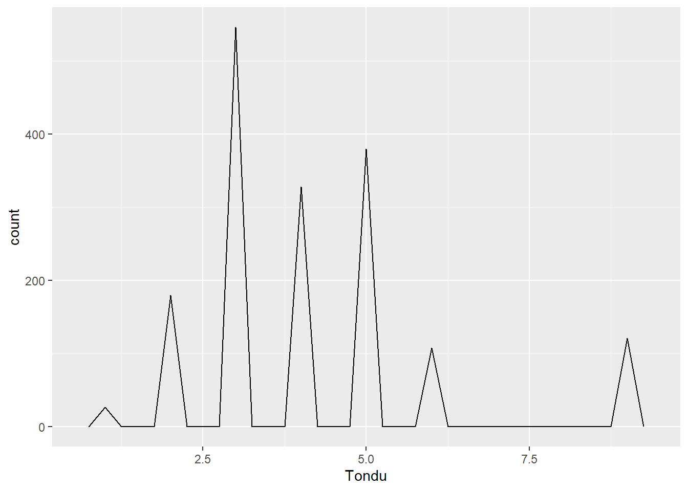
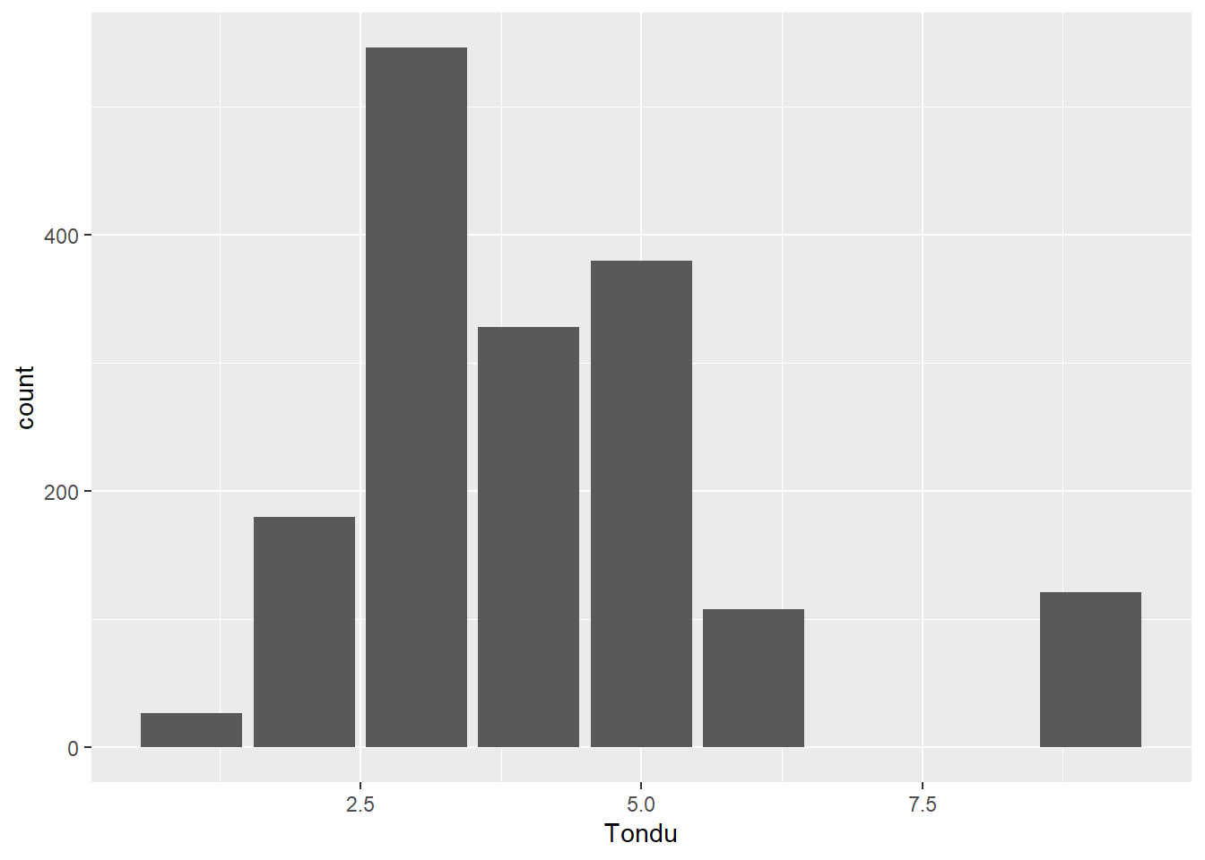
Exploring Relationship Between Tondu and Variables
ggplot(TEDS_2016, aes(x = Tondu, fill = female)) +geom_bar()
Warning: The following aesthetics were dropped during statistical transformation: fill
ℹ This can happen when ggplot fails to infer the correct grouping structure in
  the data.
ℹ Did you forget to specify a `group` aesthetic or to convert a numerical
  variable into a factor?
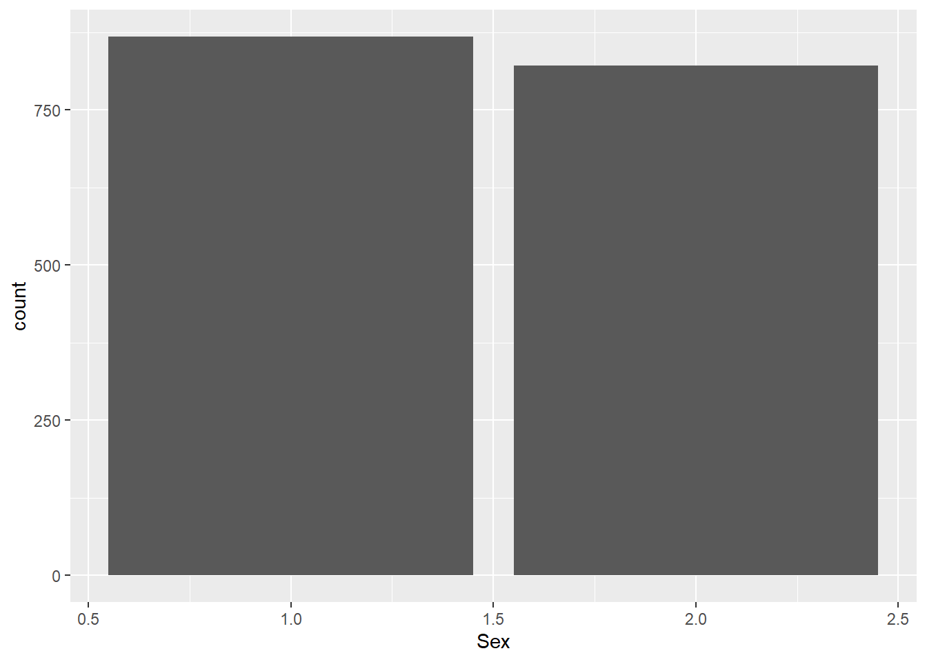
0 = Not Female (presumably male), 1 = Male
Tondu Variables:
TEDS_2016$Tondu<-as.numeric(TEDS_2016$Tondu,labels=c("Unification now”, “Status quo, unif. in future”, “Status quo, decide later", "Status quo forever", "Status quo, indep. in future", "Independence now”, “No response"))